Fourier Neural Operator 2
Micro Domain
The micro domain is defined by a bounding box and a smooth function parameterising the floor of the micro domain.
import sys
sys.path.append('/home/emastr/phd/')

import numpy as np
import torch as pt
import torch.autograd as agrad
import matplotlib.pyplot as plt
from util.plot_tools import *
from architecture.fno_1d import *
from boundary_solvers.blobs import *
from boundary_solvers.geometry import *
from scipy.sparse.linalg import gmres, LinearOperator
from operators.stokes_operator import StokesAdjointBoundaryOp
from util.unet import *
import torch.nn as nn
Create data loader
Load and transform the data.
def unpack_data(data):
    xlabels = ['x', 'y', 'dx', 'dy', 'ddx', 'ddy', 'vx', 'vy', 'w', 't']
    ylabels = ['rx', 'ry']
    inp = {xlabels[i]: data['X'][:, i, :] for i in range(10)}
    out = {ylabels[i]: data['Y'][:, i, :] for i in range(2)}
    return (inp, out)

def unpack(transform):
    """Decorator for if a method is supposed to act on the values of a dict."""
    def up_transform(data, *args, **kwargs):
        if type(data) == dict:
            return {k: transform(data[k], *args, **kwargs) for k in data.keys()}
        else:
            return transform(data, *args, **kwargs)
    return up_transform

@unpack
def subsample(x, idx):
    return x[idx]

@unpack
def integrate(x, w):
    return torch.cumsum(x * w, axis=len(x.shape)-1)

def subdict(dic, keys):
    return {k: dic[k] for k in keys if k in dic.keys()}

def concat_dict_entries(data):
    return torch.cat(tuple((d[:, None, :] for d in data.values())), dim=1)

def arclength(dx, dy, w):
    return integrate((dx**2 + dy**2)**0.5, w)

def normalize(dx, dy):
    """Normalize 2-dim vector"""
    mag = (dx**2 + dy**2)**0.5
    return dx/mag, dy/mag

def curvature(dx, dy, ddx, ddy):
    """Find curvature of line segment given points"""
    mag = (dx**2 + dy**2)**0.5
    return (dx * ddy - dy * ddx) / (mag ** 3)

def invariant_quantities(inp):
    labels = ('tx', 'ty', 'c')
    tx, ty = normalize(inp['dx'], inp['dy'])
    c = curvature(inp['dx'], inp['dy'], inp['ddx'], inp['ddy'])
    data = (tx, ty, c)
    return {labels[i]: data[i] for i in range(len(data))}
Next, we need a way to create the integral operator from a data batch.
def op_factory(inp):
    Z   = inp['x']   + 1j * inp['y']
    dZ  = inp['dx']  + 1j * inp['dy']
    ddZ = inp['ddx'] + 1j * inp['ddy']
    W = inp['w']
    a = torch.ones(Z.shape[0],) * 0.5 * 1j
    return StokesAdjointBoundaryOp(Z, dZ, ddZ, W, a)
Load Data
@unpack
def to_dtype(tensor, dtype):
    return tensor.to(dtype)

# Load and transform
data = torch.load(f"/home/emastr/phd/data/problem_data_riesz_TEST.torch")
inp, out = unpack_data(data)

dtype = torch.double
inp, out = to_dtype(inp, dtype), to_dtype(out, dtype)

# Add invariant quantities to data.
inp.update(invariant_quantities(inp))

# Normalise curvature using monotone function sigmoid(x/2) - 1/2.
inp['c'] = 1/(1 + torch.exp(-0.5 * inp['c'])) - 0.5
Split into training and test data
# Standard features (coordinates, derivatives of parameterisation)
features = {'x', 'y', 'dx','dy','ddx','ddy','vx','vy'}

# Invariant features (coordinates, tangent, curvature)
features = {'x', 'y', 'tx', 'ty', 'c', 'vx', 'vy'}

# Reduced features (trust fourier transform to handle the rest)
features = {'x', 'y', 'vx', 'vy'}


## TRAINING DATA

M_train = 200#0
M_batch = 5 # Batch
idx_train = list(range(M_train))
X_train = concat_dict_entries(subdict(subsample(inp, idx_train), features))
V_train = concat_dict_entries(subdict(subsample(inp, idx_train), {'vx', 'vy'}))
Y_train = concat_dict_entries(subsample(out, idx_train))
#X_train = subdict(X_train, {'vx', 'vy'})

## TEST DATA
M_test = 100#0
idx_test = list(range(M_train, M_test + M_train))
X_test = concat_dict_entries(subdict(subsample(inp, idx_test), features))
V_test = concat_dict_entries(subdict(subsample(inp, idx_test), {'vx', 'vy'}))
Y_test = concat_dict_entries(subsample(out, idx_test))
#X_test = subdict(X_test, {'vx', 'vy'})

in_channels = len(features)
out_channels = 2
Create network
settings = {"modes": 10,
            "input_features": features}

net = FNO1d(modes=settings["modes"], in_channels=in_channels, out_channels=out_channels)
Do training
# Predefine list of losses
trainloss = []
testloss  = []
# Loss function
loss_fcn  = nn.MSELoss()
benchloss = loss_fcn(V_test, Y_test).item()
optim     = torch.optim.Adam(net.parameters())

# DO TRAINING LOOP
##################################################
N = 30001 #30001
for i in range(N):
    idx_batch = torch.randperm(M_train)[:M_batch]
    Y_batch   = Y_train[idx_batch]
    X_batch   = X_train[idx_batch]

    # Train on truncated net that expands as iterations progress
    loss = loss_fcn(net(X_batch), Y_batch)
    loss.backward()
    optim.step()

    trainloss.append(loss.item())
    testloss.append(loss_fcn(net(X_test), Y_test).item())

    optim.zero_grad()

    print(f"Step {i}. Train loss = {trainloss[-1]}, test loss = {testloss[-1]}, benchmark={benchloss}", end="\r")

    if i % 1000 == 0:
        torch.save({"state dict" : net.state_dict(),
                    "settings"   : settings,
                    "trainloss"  : trainloss,
                    "testloss"   : testloss},
                    f"/home/emastr/phd/data/fno_adjoint_state_dict_2022_12_02_default5_{i}.Torch") # old namme unet_state_dict #Kernel size 5, stride 2
Step 30000. Train loss = 0.00014250755874667165, test loss = 0.0002593944797511047, benchmark=0.0248016101648704522
save = torch.load(f"/home/emastr/phd/data/fno_adjoint_state_dict_2022_12_02_default5_{30000}.Torch")
trainloss = save["trainloss"]
testloss = save["testloss"]
net.load_state_dict(save["state dict"])
<All keys matched successfully>
Y_net = net(X_test)
Y_net = Y_net.detach()
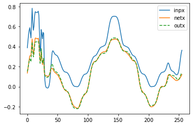
for i in [90]:
plt.figure(1)
plt.plot(V_test[i, 0, :], label='inpx')
plt.plot(Y_net[i, 0, :], label='netx')
plt.plot(Y_test[i, 0, :], '--', label='outx')
plt.legend()
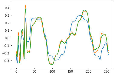
plt.figure(2)
plt.plot(V_test[i, 1, :])
plt.plot(Y_net[i, 1, :])
plt.plot(Y_test[i, 1, :])
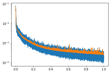
plt.figure(3)
plt.semilogy(np.linspace(0,1,len(trainloss)), trainloss)
plt.semilogy(np.linspace(0,1,len(testloss)), testloss)
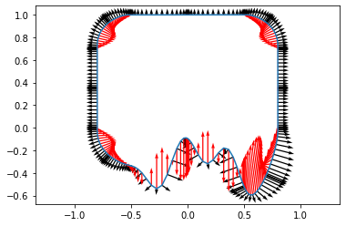
plt.figure(4)
plt.plot(inp['x'][0, :], inp['y'][0, :])
plt.quiver(inp['x'][0,:], inp['y'][0,:], inp['dy'][0,:], -inp['dx'][0,:])
plt.quiver(inp['x'][0,:], inp['y'][0,:], inp['ddx'][0,:], inp['ddy'][0,:], color='red')
plt.axis("equal")
(-0.8800000131130219,
 0.8800000131130219,
 -0.6743489861488342,
 1.0797309041023255)