HMM Stokes
Stokes Flow in Periodic Channel with Robin boundary.
import sys
sys.path.append('/home/emastr/phd/')

import torch
import time
import numpy as np
import matplotlib.pyplot as plt
from stokes2d.robin_solver import testSolve, solveRobinStokes_fromFunc
from util.plot_tools import *
from boundary_solvers.geometry import MacroGeom
Multiscale Problem
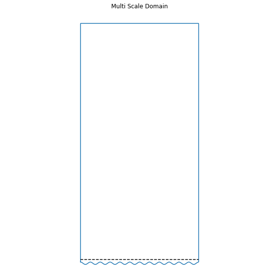
We define a multiscale problem as follows. The PDE is a non-slip zero forcing Stokes flow Problem
\[\Delta u - \nabla p = 0, \qquad \qquad \nabla \cdot u = 0 \qquad \text{inside}\quad \Omega\]with the boundary conditions
\[u = g,\qquad \text{on}\quad\partial\Omega\]the boundary is a two-dimensional pipe with corners at (0,-1) and (1,1), and a micro scale boundary:
from hmm.stokes import StokesMacProb, StokesMicProb, trig_interp, StokesData, StokesHMMProblem
from hmm.stokes import MacroSolver, MicroSolver, IterativeHMMSolver
from util.plot_tools import *

eps = 0.02
k = round(1 / eps / 4) * 4

A = 0.5
h = 1.5
f = lambda x: eps * (-h + A * np.cos(k*x)) #1.6
df = lambda x: -eps * k * np.sin(k*x) * A
ddf = lambda x: -eps * (k**2) * np.cos(k*x) * A
g = lambda x: 1+np.sin(2*np.pi * x) * 0.0
data = StokesData(f, df, ddf, g)

plt.figure(figsize=(10,10))
plt.title("Multi Scale Domain")
data.plot(plt.gca())
remove_axes(plt.gca())
plt.axis("equal")
(-0.05, 1.05, -1.1419995844364166, 1.101999980211258)
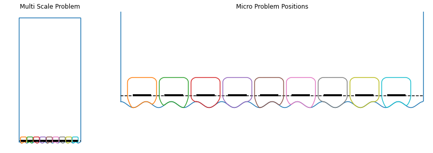
Coupling to Micro Domain
To couple the macro domain to the microscopic domain, we make use of the HMM framework. We construct a set of evenly spaced micro problems based on the Stokes data. The macro problem is constructed with a pre-specified resolution in the x- and y-directions.
# Macro problem
xDim = 21
yDim = 23
iDeg = 13 #nMic*2 +1
macro = StokesMacProb(data, lambda x,a: trig_interp(x,a, iDeg))

# Micro problems
nMic = 9
xPos = np.linspace(4*eps, 1-4*eps, nMic)-2*eps
micros = [StokesMicProb(data, x, 3*eps, 3*eps, 0.01) for x in xPos]

# Hmm problem.
hmm_prob = StokesHMMProblem(macro, micros, data)

## PLOT ##

plt.figure(figsize=(15,5))

plt.subplot2grid((1,4), (0,0), colspan=1)
plt.title("Multi Scale Problem")
hmm_prob.plot(plt.gca())
plt.axis("Equal")
remove_axes(plt.gca())

plt.subplot2grid((1,4), (0,1), colspan=3)
plt.title("Micro Problem Positions")
hmm_prob.plot(plt.gca())
plt.axis("Equal")
remove_axes(plt.gca())
plt.xlim([-eps,1 + eps])
plt.ylim([-1-1*eps, -1+6*eps])
(-1.02, -0.88)
Solving using HMM iterations
To solve the problem, we make use of a sequence of micro solvers, as well as a micro solver.
class Callback():
    def __init__(self, macro):
        self.N = 100
        self.x = np.linspace(0,1,self.N)
        self.macro = macro
        self.current_alpha = macro.alpha(self.x)
        self.diff = []

    def __call__(self, it, macro_sol, micro_sols):
        self.previous_alpha = self.current_alpha
        self.current_alpha = self.macro.alpha(self.x)
        self.diff.append(np.linalg.norm(self.previous_alpha - self.current_alpha) / self.N**0.5)

debug_cb = Callback(macro)

print("Precomputing...")
macro_solver = MacroSolver(xDim, yDim)
micro_solvers = [MicroSolver(m) for m in micros]
hmm_solver = IterativeHMMSolver(macro_solver, micro_solvers)
print("Done")


print("HMM Solver...")
macro_guess = macro_solver.solve(macro)
(macro_sol, micro_sols) = hmm_solver.solve(hmm_prob, macro_guess=macro_guess,
                                           callback=debug_cb, verbose=True, maxiter=7)
print("\nDone")
Precomputing...
Done
HMM Solver...
Step 6/7
Done
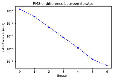
Convergence study for slip coefficient
plt.figure()
plt.title("RMS of difference between iterates")
plt.semilogy(debug_cb.diff, 'b*--')
plt.xlabel("Iterate n")
plt.ylabel("RMS of a_n - a_(n+1)")
Text(0, 0.5, 'RMS of a_n - a_(n+1)')
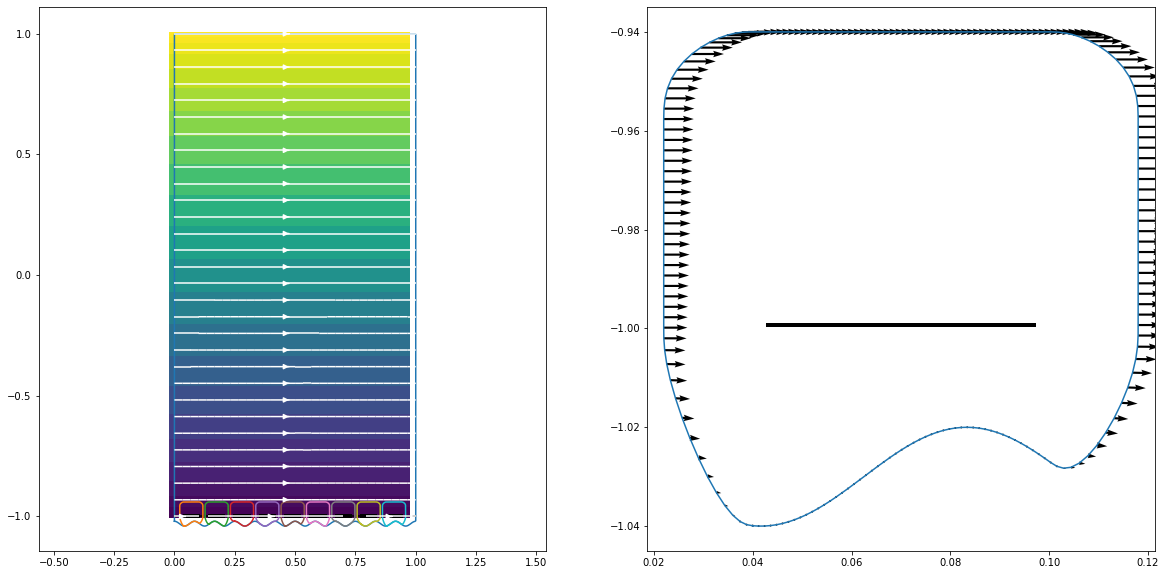
plt.figure(figsize=(20,10))
plt.subplot(121)
plt.axis("equal")
hmm_prob.plot(plt.gca())
macro_sol.u.plot(plt.gca())
macro_sol.plot_stream(plt.gca(), color="white")
plt.subplot(122)
micros[0].plot(plt.gca())
micros[0].geom.plot_field_on_boundary(plt.gca(), micros[0].condition)
plt.axis("equal")
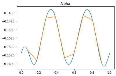
plt.figure()
plt.title("Alpha")
x = np.linspace(0,1,100)
a = macro.alpha(x)
xm = np.array([sol.x for sol in micro_sols])
am = np.array([sol.alpha for sol in micro_sols])
plt.plot(x, a)
plt.plot(xm, am)
#print(macro.alpha)
#plt.figure(figsize=(10,6))
#plt.title("Condition")
#t = np.linspace(0,2*np.pi, 300)
#v = micros[0].condition(t)
#plt.plot(t, np.real(v))
#plt.plot(t, np.imag(v))
#plt.xlim([1,3])
[<matplotlib.lines.Line2D at 0x7fa5cd550100>]
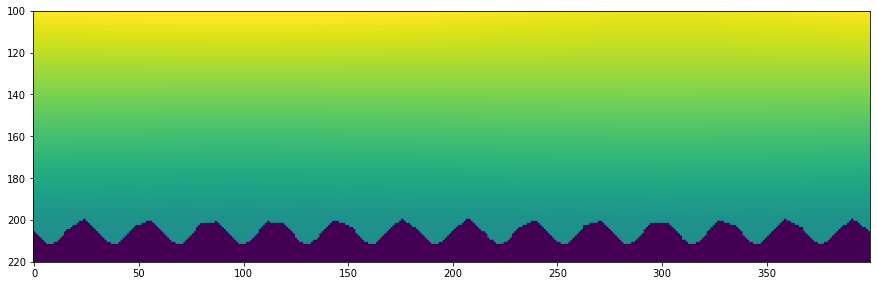
from scipy.io import loadmat
import matplotlib.pyplot as plt

matf = loadmat("/home/emastr/phd/data/reference/run_24.mat", struct_as_record=True)
info = matf['info'][0][0]
Uc = info['Uc']
Vc = info['Vc']
mask = np.isnan(Uc)
Uc = np.where(mask, -np.ones_like(Uc), Uc)
X = info['X']
Y = info['Y']

plt.figure(figsize=(15,5))
plt.imshow(Uc[::-1, ::-1], vmin=-0.5, vmax=0.5)
plt.ylim([220, 100])
(220.0, 100.0)